k-Means with exhaustive constraints

In the following code, we give an example for constrained spectral clustering on a toy grid dataset using different exhaustive size constraints.

We start by creating a data point which form a uniform 2D grid:

import matplotlib.pyplot as plt
import numpy as np
from ccluster.size import constrained_k_means

# generate a uniform grid
nx = np.arange(0, 100, 5)
ny = np.arange(0, 100, 5)
x_coords, y_coords = np.meshgrid(nx, ny)

data = np.column_stack([x_coords.reshape(-1), y_coords.reshape(-1)])

Assume we wish to partition this grid into 4 groups with different cluster distributions. The \(k\)-means algorithm is a good choice for this kind of data. We create these different distributions as follows:

n_clusters = 4

constraints = [
    [100, 100, 100, 100],
    [200, 120, 40, 40],
    [260, 120, 10, 10]
]

These constraints are exhaustive in the sense that each constraint list sums to the total number of data points in the grid and there are 4 values in each list, one for each cluster.

Finally, we run the algorithm for each different constraint and create plots for the results:

for cluster_size in constraints:
    _, labels, _ = constrained_k_means(data,
                                       n_clusters=n_clusters,
                                       cluster_sizes=cluster_size)

    # plotting
    plt.figure(figsize=(6, 6))
    plt.scatter(data[:, 0], data[:, 1], c=labels)
    plt.xlabel('X')
    plt.ylabel('Y')
    plt.axis('off')

    plt.title(f'{n_clusters} clusters with sizes {*cluster_size,}')
    plt.show()

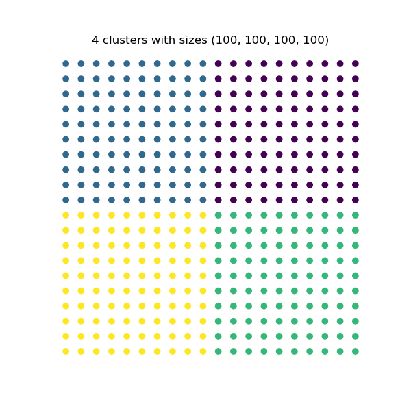
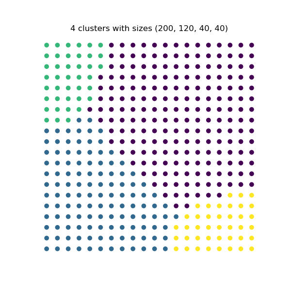
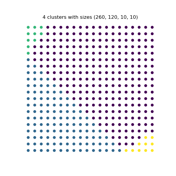
We see how each resulting partition respects its corresponding constraint exactly.

Spectral clustering with partial constraints

The following example shows an example for constrained spectral clustering on a toy spiral dataset for different cluster partial size constraints.

We start by creating the 2D spiral:

import matplotlib.pyplot as plt
import numpy as np
from ccluster.size import ConstrainedSpectralClustering

# generate a spiral
x_coords = []
y_coords = []

for theta in np.linspace(7, 10 * np.pi, 400):
    r = theta ** 2
    x_coords.append(r * np.cos(theta))
    y_coords.append(r * np.sin(theta))

data = np.column_stack([x_coords, y_coords])

We then create a set of different constraints for our algorithm for partitioning the spiral into 4 clusters.

n_clusters = 4

constraints = [
    [100, 100],
    [5, 5],
    [388]
]

Since this data is in a spiral, constrained spectral clustering is a better choice than \(k\)-means to create a nearest neighbors graph and generate a different partition for each constraint. At the end, we plot the results:

for cluster_size in constraints:
    labels = ConstrainedSpectralClustering(
        n_clusters=n_clusters,
        cluster_sizes=cluster_size,
        affinity='nearest_neighbors',
        n_neighbors=2
    ).fit_predict(data)

    # plotting
    plt.figure(figsize=(6, 6))
    plt.scatter(data[:, 0], data[:, 1], c=labels)
    plt.xlabel('X')
    plt.ylabel('Y')
    plt.axis('off')
    plt.title(f'{n_clusters} clusters of which {len(cluster_size)} have sizes {*cluster_size,}')
    plt.show()

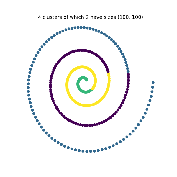
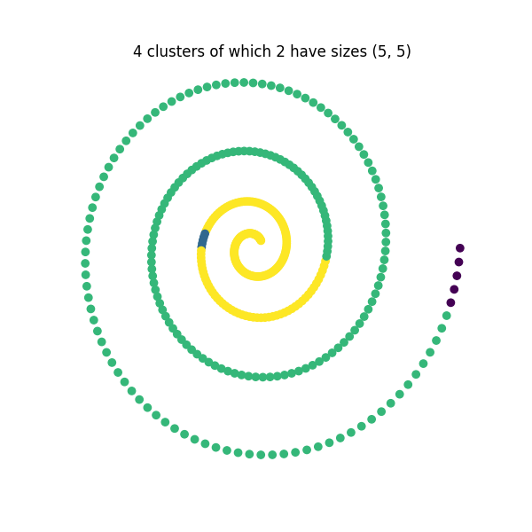
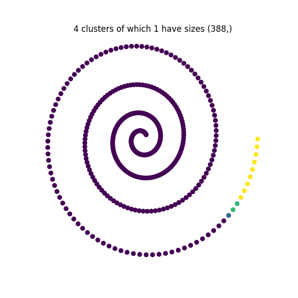
We see how in each case, there exists clusters with the desired sizes while the remaining cluster sizes are free.